Expected results from a game of Beetle


Beetle

beetle

With the holidays coming up, it’s time for family reunions and dice-games. In my family, we play a game called Beetle. It’s a very simple dice-game, relying solely on random chance, requiring no skill to play. The objective is to finish drawing your Beetle first. A beetle consists of:

  • A body
  • A head
  • A tail
  • 2 eyes
  • 2 antennae
  • 6 legs

You take turns rolling a die, with each number of eyes corresponding to a body part. They are paired as:

  1. Tail
  2. Eyes
  3. Antennae
  4. Legs
  5. Head
  6. Body

A beetle is built from the inside out – that is, you can’t draw the legs, tail or head before you have drawn the body, and you can’t draw the eyes or the antennae before you have drawn the head.

The winner of a round is the first person to complete their beetle. After a winner is announced, no more dice can be rolled and the round stop. Then everyone tally up the score of their beetle and continue unto next round. Usually a game consists of 10 rounds, after which the overall winner is the person with the highest total score.

A beetle is scored based on how complete it is. Each body part is worth as much as the die-value associated with it. So a body is worth 6, a head 5 and so on… A complete beetle has a score of 46.

Expected results

Having an analytical mind, I couldn’t help but think what the average game of Beetle looked like. Is 316 a good final score? What are the chances of getting 0 points in a round?

Naturally, I had to simulate lots of Beetle games to get some data to work with. Luckily, the game is entirely based on chance, so there’s no fiddling with an AI to get this to work. I made an implementation in Java, which can be seen on its GitHub page, though I won’t detail how it works in this post.

In my family, we are ~25 people playing Beetle at once, in groups of 3-4 people with each group having one die. Having multiple dice in this game is an illusion, because any two dice-rolls will never occur at exactly the same time. Thus, any game with multiple dice could be simulated using a single die moving in a strange pattern between the players.

Anyway, I simulated 10mio. games and got some results:

[0.058]   Simulating 10.000.000 games (pop. 25)...
[460.066] Analyzing...
[612.833] SCORES
Median:           30
Max:              46
Arithmetic mean:  29.35860358
Variance:        102.34945493498675 (std = 10.11679074286835)
[612.834] GAME LENGTH
Median:           20
Max:              35
Arithmetic mean:  19.9951173
Variance:          7.044919563914728 (std = 2.6542267355888662)

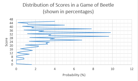
The median score is 30. Whenever I’ve played this game I used to think 30 was a good score, but I guess I was wrong. Let’s take a look at the distribution of the scores in game of Beetle (I’m using a population size of n=25):

Capture

cdf


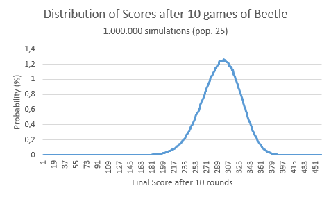
10games

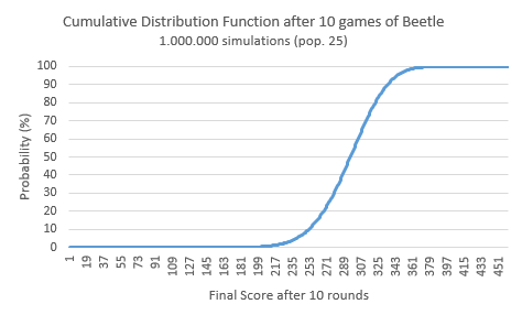
cdf 10


Golden ratio and Fibonacci


I’m currently doing a course on linear algebra, and while working on a hand-in, I discovered this neat proof that the Fibonacci sequence grows exponentially.

Definition: Define two sequences:

  1. a_1 = 1, a_2 = 3, \text{ and } a_n = a_{n-1} + a_{n-2} \text{ for } n>2
  2. b_1 = 1, b_2 = 1, \text{ and } b_n = b_{n-1} + b_{n-2} \text{ for } n>2

Notice that b corresponds to the Fibonacci sequence, and a corresponds to the Lucas numbers, first index truncated.

Lemma 1: For all k>0

  1. a_k = \frac{1}{2} \left ( a_{k-1} + 5\cdot b_{k-1} \right )
  2. b_k = \frac{1}{2} \left ( a_{k-1} + b_{k-1} \right )

Proof. Shown only for 1.1, the proof is similar for 1.2. Proven using strong induction on k.

  • Base-case: 
    Notice that \frac{1}{2} \left ( a_{0} + 5\cdot b_{0} \right ) = \frac{1}{2} \left ( 1 + 5\cdot 1 \right ) = \frac{1}{2} \left ( 6 \right ) = 3 = a_1.
    Which is what we wanted to show.
  • Induction: 
    We see a_k = a_{k-1} + a_{k-2}, by definition.
    We apply the induction hypothesis on k-1, and k-2 to get: a_k = \frac{1}{2} \left ( a_{k-2} + 5\cdot b_{k-2} \right ) + \frac{1}{2} \left ( a_{k-3} + 5\cdot b_{k-3} \right ). We use the definition of a_k and b_k, and get
    a_k = \frac{1}{2} \left ( a_{k-1} + 5\cdot b_{k-1} \right ). Which is what we wanted to show. \blacksquare.

Lemma 2: For all k>0\phi^k = \frac{1}{2} a_k + \frac{1}{2} b_k \cdot \sqrt{5}.

Proof. We prove this lemma using induction on k.

  • Base-case:
    We see that, \frac{1}{2} a_1 + \frac{1}{2} b_1 \cdot \sqrt{5} = \frac{1}{2} 1 + \frac{1}{2} 1 \cdot \sqrt{5} = \frac{1}{2} \left(1 + \sqrt{5} \right) = \phi. Which is what we wanted to show.
  • Induction step:
    We get \phi^k = \phi \cdot \phi^{k-1} = \frac{1}{2}(1+\sqrt{5})\cdot \left( \frac{1}{2} a_{k-1} + \frac{1}{2} b_{k-1} \cdot \sqrt{5} \right), using the induction hypothesis. Multiplying, we get \phi^k = \frac{1}{2} \left ( \frac{1}{2} \left ( a_{k-1} + 5 b_{k-1} \right ) \right ) + \frac{1}{2} \left ( \frac{1}{2} \left ( a_{k-1} + b_{k-1} \right ) \right ) \cdot \sqrt{5}. Using lemma 2, we find \phi^k = \frac{1}{2} a_k + \frac{1}{2} b_k \cdot \sqrt{5}, which is what we wanted to show. \blacksquare.

Now for the interesting part of this article:

Theorem: b_n = \Theta(\phi^n).

Proof. We split the proof into two parts; first proving that b_n = O(\phi^n), then proving b_n = \Omega(\phi^n).

  • b_n = \Omega(\phi^n).
    We see that \phi^n < \frac{1}{2} a_n \cdot \sqrt{5} + \frac{1}{2} b_n \cdot \sqrt{5}, because of lemma 2. Because of lemma 1.2, we have b_n = \frac{1}{2} a_n + \frac{1}{2} b_n, so we get \phi^n < b_{n+1} \cdot \sqrt{5}. This implies that b_n = \Omega(\phi^n).
  • b_n = O(\phi^n).
    We see that \phi^n > \frac{1}{2} b_n because of lemma 2, which implies that b_n = O(\phi^n).

Because b_n = O(\phi^n), and b_n = \Omega(\phi^n), we have b_n = \Theta(\phi^n). That is, the Fibonacci sequence grows exponentially, with base \phi. \blacksquare.

Calkin-Wilf Fractals


Suppose we have two natural numbers i,j. Define a sequence a_0 = i, a_1 = j and a_n = |a_{n-1} - a_{n-2}|. That is, we start with two initial values, and repeatedly subtract the smallest value from the largest value. Since i,j \geq 0, we know that a_n \geq 0 for all n.

Eventually, we will reach the cycle \ldots 1, 1, 0, 1, 1, 0 \ldots no matter our choice of i,j (to see why, consider the termination function \mu(i,j)=i+j and the invariant that any term must be positive).

Define

\text{chainLength}(i,j) = \text{largest } n \text{ such that } a_n \notin \{1, 0\}

We can now make pretty pictures. For each pixel (x,y) color pixel by \text{chainLength}(x,y) which can be calculated using a simple recursive procedure:

int chainLength(int x, int y){
 if(x == y || x==0 || y==0)
     return 0;
 if(x>y)
     return 1+chainLength(x-y,y);
 else
     return 1+chainLength(x,y-x);
 }

calkinwilf

Generated using the DELTA library.

Connection to Calkin-Wilf trees

The Calkin-Wilf tree is an infinite binary recursive tree, where the root node is defined as 1/1, and every node a/b has a left child \dfrac{a+b}{b} and right child \dfrac{a}{a+b}.


capture

The Calkin-Wilf tree is useful because it allows us to define a bijection between the natural numbers and the rational numbers, which can be used to show that the rational numbers are a countably infinite set.

Notice that if a node x/y is a left child, then x>y, and if it’s a right child then y > x. This allows us to determine the parent node of a given node.

If for a given node x>y then we know it was the left child of its parent. So we know its parent is (x-y) / y. Similarly, if y>x, then its parent is x/(y-x). Notice that at each step, we subtract the smaller number from the larger number, and we terminate the procedure when we reach the fraction 1/1.

Going back to a_n, we could interpret a pixel (x,y) as the rational number x/y. The recursive sequence \text{chainLength}(x,y) would then be equivalent to the depth of the node $latex x/y$ in the Calkin-Wilf tree.

Keep in mind that the Calkin-Wilf tree only contains rational numbers in the lowest common term, so the node 2/2 does not exist in the Calkin-Wilf tree. To circumvent this issue, we convert our input node to the equivalent rational number in lowest common terms.

Incendium – HTML 5 App


fractal22

I just realized I have had this app up for a while on my github.io without posting it here. Anyway, I made an HTML5 app which implements the algorithm detailed in my previous post on fractal animations.

Moving the mouse around on the screen changes two different parameters, with each point P corresponding to a unique configuration.

http://ssodelta.github.io/incendium/

It is written for Google Chrome, and is known to act weird on Firefox sometimes. It may also crash, but just restart the page (sry).

AIArena – Bot Tournament


AIArena is a tournament where contestants write scripts for bots which battle each other in a virtual arena. I have written a dynamic web application which allows users to submit their own bots, written in a custom imperative scripting language dubbed BOTScript. The server will itself make the bots battle each other, ranking them on the website by how many wins each bot gets.

AIArena website: http://dank.business.com/bots/

GitHub: https://github.com/SSODelta/BotBrawl

If you have ideas, suggestions, feedback, criticism or whatever, drop me a line at admin@ssodelta.com.

Sample of the DELTA Library


The DELTA library

If you look through my blog, you’ll find posts where I detail an algorithm for making fractals, or other visually appealing animations/images. To aid myself in the future, I have written a library for Java8 which contains some nice classes and operations for manipulating colors and images.

You can take a look at it at its GitHub page (contains a README.md), though I will detail with the library with further scrutiny on this blog at some point in the future (studying is keeping me busy atm):

https://github.com/SSODelta/DELTA

Often when making single images, there are some dimensions you can change to produce animations. I thought two previous posts were especially suitable for this, so I have made two very nice animations, imo:

Newton Fractals

The biggest problem with animating this fractal, was that I lost the information about which root was assigned which colors when slighting altering the parameters of the polynomials. Instead, using DELTA I have colored each root r_0 using HSV colors with hue proportional to the argument \mathrm{arg}(r_0) and the number of iterations it took for the point to converge – and saturation/value decreased with increasing magnitude |r_0|.

Regex Fractals

Here, the hue is proportional to the edit distance and the time t, and saturation/value inversely proportional to only the edit distance.

Ludum Dare 34


12375456_10207058414872353_2058174363_o

I was convinced by some of my friends to participate in this year’s Ludum Dare. If you’re unfamiliar with the concepts, it’s a game jam – so you have to develop a video game from start to finish in a very limited time frame. In this case, we had 72 hours to develop our idea.

We chose to go with the theme “2 Button Controls” (this year had two possible themes) and developed a simple arcade fighting game à la Street Fighter. I did most of the programming, and my friend Thomas did the graphics, audio and design of the project. I’m very pleased with the result, it is the first game I have started in Unity that I’ve actually finished – most likely because of the short time span.

The code is unstructured, disorganized, fragmented and written pretty poorly. But it has go fast when you’re a jam – it’s not so much about creating the perfect piece of code art, it’s about getting shit done and getting it done fast. I had a lot of fun with this, and will definitely be participating in future jams.

Ludum Dare link: http://ludumdare.com/compo/ludum-dare-34/?action=preview&uid=66145

Play online (requires Unity WebPlayer): https://dl.dropboxusercontent.com/u/19633784/web.html

Download as executable (.exe): https://dl.dropboxusercontent.com/u/19633784/ld34.zip

Source code (Unity project): https://github.com/SSODelta/LudumDare34

LoGiX v1.1.1


LoGiX has been updated to a new build and includes some nice new features and small bug-fixes. Here is the changelog:

Added support for {...} statements and line-breaks;
Added support for in-line comments.
Added support for comments if the output is false.
Improved loading system.

Added support for {…} statements and line-breaks;

The most nice new feature is the curly brackets. I used to have this implemented, but when I rewrote the engine entirely once, I lost feature. But it’s really cool, basically, you type a list list {a,b,c}, and then the LoGiX-engine will replace the curly brackets with each element inside it. So we can type

:> def {P,Q}

Which evaluates as:

:> def P
:> def Q

Which saves a lot of space in programs. A nice example is modus ponens, which before was written as:

:> !def P
:> !def P implies Q
:> Q?
true

Using the new notation, we can write:

:> !def P {,implies Q};Q?
true

Which is very cool! I think this is the shortest you can write modus ponens in LoGiX. It is of course possible to do these multiple places in the command, so we get:

:> def {P,Q,R} implies {A,B}
def P implies A
def Q implies A
def R implies A
def P implies B
def Q implies B
def R implies B

Added support for in-line comments.

Another new feature is the ability to do inline comments. Before, the compiler would crash if a #-symbol appeared not at the beginning of a line. But now, it treats everything after the #-symbol as a comment.

:> def P #Now we've just defined P and made a comment
def P

Added support for comments if the output is false.

And now it’s also possible to use custom messages when the output is false. Before we could do:

:> def {P,Q} implies R
:> def P or Q
:> R?its true
its true

It interprets whatever is after the question mark as the message it prints if the statement is true. However, it was not possible to do the same if the statement was false – it would always return ‘false‘. But now you can do this too:

:> def P and Q implies R
:> def P or Q
:> R?its true|definitely not true
definitely not true

Incendium – Making fractal animations


Udklip

I’ve recently created a piece of software for creating fractal animations. The full source code and a description of its features can be found at the project’s GitHub page. On this page, however, I’ll explain the technical details behind the algorithm used by the core engine of Incendium to generate its fractals. If you want a non-technical overview, please check out the GitHub page. In essense, the program works by drawing a bunch of polygons unto an empty frame. There are two central problems here, how to choose which polygons to draw, and to figure out where to draw them.

We start with a regular n-gon (called depth d=0) drawn with its center at the origin (0,0), and from each of its vertices, we draw another regular n-gon (it does not need to be the same n for every depth). These new polygons have center at the vertices of the old polygon and have depth d=1, and in general a polygon at depth d=n will have children of depth d=n+1. We continue doing this process until we’ve reached the specified fractal depth, giving us images such as (shown from depth d=0 to d=2):

naming_regex_tri_noname

Note that this image uses triangles, rather than the more general n-gon. This is because the math is pretty much the same for any n, and triangles are easier to visualize. Note that we’ve drawn all triangles here – what is a good method to choose which of these triangles to choose?

Choosing which polygons to draw

First of all, let’s label the polygons accordingly in a systematic fashion. Let’s label the very first n-gon the empty string \epsilon. Its n children will be appended the characters \Sigma = \{0,1,2,...,n-1\}, meaning that the children of the root node are called 0,1,2,...,n-1. The children of the polygon represented by the string 0 will likewise be appended these characters, and thus be called 00, 01, 02, ..., 0n. Adding these labels to the above drawing yields:

naming_regex_tri

Note that the length of the string s is directly related to the depth of the polygon represented by that string, that is |s|=fd for some fractal depth fd. For a constant polygon degree throughout the fractal, we will have a polygon for every possible string s \in \Sigma^* : |s| \leq fd. Thus we’ve reduced the problem of determining which polygon to draw to choosing a language L \subset \Sigma^* and drawing all the polygons represented by the strings in L. Please note that since the polygon degree isn’t necessarily constant, we can’t be sure that all such strings s actually exist in the fractal, but there is a relatively simple workaround.

To do this, we employ the help of regular expressions. While this technically limits the class of possible languages, it is a very simple approach, so we’re sticking with it. So, given some regular expression R we draw all polygons represented by all the strings in L(R). Shown here is the regular expression .^*1.^* which only accepts all regular expressions that contain a 1:

naming_regex_tri_only1

Where do we draw them?

single-polygon

Still, it’s not enough to just know which polygons to draw, we also need to know where to draw them. The root polygon is by definition placed at (0,0), so its location is trivial. It’s children are drawn with their centers at the vertices of the root polygon, which seems to suggest we need the position of these. Assume we have some polygon with “radius” r and rotation \theta. We know that all the vertices of the polygon lie on the graph for the circumscribed circle of the polygon. Therefore, we can easily derive the following formulas for the position of the vertices using trigonometry:

P_0 = ( r \cdot \cos(\theta), r \cdot \sin(\theta) )

P_1 = \left ( r \cdot \cos( \theta + \frac{1}{n} \cdot 2 \pi), r \cdot \sin( \theta + \frac{1}{n} \cdot 2 \pi) \right )

P_2 = \left ( r \cdot \cos( \theta + \frac{2}{n} \cdot 2 \pi), r \cdot \sin( \theta + \frac{2}{n} \cdot 2 \pi) \right )

And in general,

P_k = \left ( r \cdot \cos( \theta + \frac{k}{n} \cdot 2 \pi), r \cdot \sin( \theta + \frac{k}{n} \cdot 2 \pi) \right )

Where P_k is the k-th vertex.

Now, assume we have some polygon at depth d represented by some regular expression R=a_0 a_1 a_2 ... a_k, and we want to know the position of its vertices. We know the origin of this polygon is given by the polygon at depth d-1. This other polygon is naturally represented by the regular expression R' = a_0 a_1 a_2 ... a_{k-1}, so its position is P_{R'}. We know the character a_n represents which vertex we have (0 being the first vertex, 1 being the next vertex etc.). Therefore, we can write the following recursive relation:

P_{a_0 a_1 a_2 ... a_k} = P_{a_0 a_1 a_2 ... a_{k-1}} +  \left ( r(R) \cdot \cos( \theta(R) + \frac{a_k}{n} \cdot 2 \pi), r(R) \cdot \sin( \theta(R) + \frac{a_k}{n} \cdot 2 \pi) \right )

 Where r(R) is the radius for the polygon represented by R, and \theta(R) is the angle – these will be investigated later. This recursive relation has the base-case P_\epsilon = (0,0) and implementing it is straight-forward (shown here in pseudo-code):

function positionFromRegex(R)
    if len(R) == 0: return (0,0)

    return positionFromRegex(R')
           + ( r(R) * cos(theta(R) + a_k/n * 2pi),
               r(R) * sin(theta(R) + a_k/n * 2pi) )

It’s the size that matters

In the previous section, we just used r(R) to denote the radius of the polygon represented by the regular expression R, we’ll now derive an expression for this function. First note that the size should only be dependent on the depth. Strings of the same depth should have the same size – we don’t want 0210 to be larger than 1203. Therefore, we can assume that the argument for r is a number, so we have r(d) : d \in \mathbb{N}. Obviously, we want r(0) to be the largest radius (for the root polygon), and we label this r_0, so r(0) = r_0. We also want this function to be strictly decreasing as n \rightarrow \infty, so r(d) > r(k) for every d > k. Finally, we want to structure we’re designing to be a fractal – it should converge towards the same points as n \rightarrow \infty.

Note that the maximum distance from the origin that the first polygon can get is r(0), and therefore the maximum distance any polygon at depth d=1 can get from the origin is r(1) and so on… Therefore the maximum distance any polygon at an arbitrary depth d can get is r(0) + r(1) + ... r(d). And since we want our fractal to be finite we require this sum to be finite, that is:

\displaystyle \sum_{d=0}^{\infty} r(d) = K

For some finite constant K \in \mathbb{R}. This looks an awful lot like infinite geometric series. While it’s not the exclusive solution for r, it is a possible one giving us the following expression for r(d):

r(d) = r_0 \cdot \rho^d

For some constant \rho \in [0,1]. We call this constant the size decay of the fractal.

You spin my head right round…

We’ve just derived the expression for the function r(R) and now we’ll do the same for \theta(R). Using a similar argument as in the previous section, we want the argument of \theta to be the length of the regular expression R. We also want the rotation to not be very chaotic, as the assumption is that this won’t create beautiful fractals. Therefore we want the fractals to rotate a constant amount at every subsequent depth. This means we can derive the following expression for \theta(n):

\theta(n) = \theta_0 \cdot n

Where \theta_0 \in [0, 2\pi] is a constant. We call this constant the rotation of the fractal.

Putting it all together

Now we’ve derived expressions for the two unknown functions and we get the following final recursive relation for the position P of a polygon represented by the regular expression R= a_0 a_1 a_2 ... a_k:

P_{a_0 a_1 a_2 ... a_k}[x] = P_{a_0 a_1 a_2 ... a_{k-1}}[x] + r_0 \cdot \rho^k \cdot \cos( \theta_0 \cdot k + \frac{a_k}{n} \cdot 2 \pi)

P_{a_0 a_1 a_2 ... a_k}[y] = P_{a_0 a_1 a_2 ... a_{k-1}}[y] + r_0 \cdot \rho^k \cdot \sin( \theta_0 \cdot k + \frac{a_k}{n} \cdot 2 \pi)

P_\epsilon = (0,0)

I’ve split it into two lines for and to make it more comprehensible. We can also write this in pseudo-code:

function positionFromRegex(R)
    k = len(R)
    if k == 0: return (0,0)

    return positionFromRegex(R')
           + ( r_0 * rho^k * cos(theta_0 * k + a_k/n * 2pi),
               r_0 * rho^k * sin(theta_0 * k + a_k/n * 2pi) )

This has been implemented in the source code in the function called getPositionFromString();.

Recursively Generating Gradient Images from Regular Expressions


I’ve decided to write yet another blog post on this blog post (first post, second post), because I’ve found another algorithm which is far superior to the other algorithms. I’ve almost completely rewritten the source code (which can be found at this project’s GitHub page). Using this approach I’ve been able to generate a 16.384px x 16.384px image (right click > save as, my browser crashes trying to render the image).

172088341

The Problem

The greatest problem with the old algorithm was that we had to enumerate all strings, check if they’re part of the regular language and then compute their Hamming distances using @nya’s O(n) algorithm, which works much better than the modified O(n^2) algorithm for Levenshtein distance previously used. But since there are 4^d strings for some depth d this whole procedure quickly becomes infeasible as especially testing for membership in the regular language is expensive. This makes rendering the images very slow.

Another fatal problem with the old algorithm was its memory usage. For instance, for d=13 (images of size 8192px x 8192px) we need to save 67 million strings and equally many pixels. To calculate how much memory that many strings will take up on the heap, we can refer to the article on Javamex (since I’ve written the program in Java, results may be different for C++, Pascal, etc.), which states that the minimum number bytes B a single string of length n takes up on the heap is:

B = 8 \cdot \left \lceil \dfrac{n \cdot 2 + 45}{8} \right \rceil

Which for d=13 gives 5.0 GB of heap usage. Similarily, a BufferedImage uses 4 bytes of information per pixel and has 4^{13} pixels in total, resulting in a heap usage of 256 MB. This is all very inefficient and is a huge, unnecessary drag on the system. It also sets a strict upper bound on the size of the images as all this memory allocation quickly becomes too much for the size of the RAM in the computer. For my computer (which has 8 GB of RAM) this strict upper bound is d=14, as it would require 21 GB of memory to store both the image and the strings.

Fortunately, there is a way around most of this, and that is what we’ll be discussing in this article. Essentially, what we do is enumerate the strings one by one and add them to the image immediately, rather than generate all of them. We also circumvent the problem of testing for membership using a clever construction.

The Algorithm

To fully understand how this algorithm works, it’s essential to have some preliminary knowledge of finite automata and regular languages. A regular expression defines a regular language L, and so do finite automata. We can therefore construct a finite automaton from a regular expression. To do so, we employ the help of the dk.brics.automaton package written by Anders Moeller from Aarhus University. The reason we use finite automata is that they have a lot of nice features – there are efficient algorithms to minimize automata and determine language membership of strings.

What we want, however, is not the language that is defined by the regular expression – we want to restrict the strings to have a length d given some depth. Therefore we can compute the intersection of the automaton that accepts strings of length d and the automaton which defines L. Next up, we’ll enumerate all strings in L \cap \Sigma^d and store them in an array M.

Other than having an automaton A_1 which recognizes strings of length d in L, we also want an automaton A_2 that recognizes all strings of length d which aren’t in L – this is just L^c \cap \Sigma^d. Because now that we have M, we want to assign the remaining strings recognized by A_2 distances and save the associated pixel information in our raster.

To do this, we perform a depth-first search of A_2, starting at some initial state S. This can be written in Java-like pseudo-code as:

process(State s, String currentString, int depth){
    //Stop at end nodes
    if(depth == max && s.isAccepted()){
        int dist = getHammingDistance(s);
        paintPixel(currentString, dist);
        return;
    }
    
    //Otherwise, get all transitions and process them as well
    for(Transition t : s.getTransitions()){
        process(t.getDestination(), currentString+t.getChar(), depth+1);
    }
}

The most obvious speed-up with this approach is that s.isAccepted(); is a cheap operation, whereas testing for membership of a string in a regular language has a worst-case time complexity of O(e^n). The other advantage is that there is no reason to save all the Strings in an array, making it possible to make much larger images. To view the algorithm in further detail I encourage you to go read the source code for this project (there is decent documentation, so the code shouldn’t be too difficult to read).

Gallery

While there are plenty of these images in the previous posts, I thought it’d be fun to share a few more of them.

489401655 239796234 610459308 737665762 806638930 831050543