solution – SSOΔ

Fractals have always amazed me. Every time I see a fractal, I can get just as excited as the first time I saw the mandelbrot set. In this post, we’ll go through a method, which can generate beautiful structures from simple functions.

Link to the source code for this project: https://github.com/SSODelta/newtons-fractals

For a real-valued function $f(x)$ , a root is any $x$ , which satisfies $f(x) = 0$ . A trivial case might be $x=0$ for the function $f(x) = x^2$ . Roots are also what is found with the famous solution $\frac{-b \pm \sqrt{D}}{4\cdot a \cdot c}$ to the quadratic equation $f(x) = a \cdot x^2 + b \cdot x + c$ .

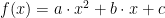
Sometimes however, a second degree equation does not have any real solutions. That is when $D < 0$ . A quadratic equation will, however always have two solutions in the complex plane.

The complex plane is an extension of the real number line to a plane. The major new addition is the introduction of the imaginary unit $i$ , which is the unique number satisfying $i^2 = -1$ . This allows us to find solutions to equations such as $x^2 = -1$ , which otherwise wouldn’t have any real solutions. In the complex plane every single point has a unique complex number associated with it. A complex number consists of two parts, a real part and an imaginary part. This is usually stylized $a + b \cdot i$ , where $a$ is the real part and $b$ is the imaginary part.

What does all this have to do with fractals?

To make a fractal, we need to assign a color code to each point in a plane, in this case the complex plane as discussed above. We decide on an initial size $(w, h)$ and a resolution $r$ . The size is the width $w$ and height $h$ of an image measured in pixels. The resolution $r$ is the “zoom-factor”, if you will. If $r=1$ , then we’ll deal with complex numbers $a + b \cdot i$ in the range $a,b \in [-1, 1]$ . And in general $a,b \in [-r, r]$ . To make it clear how to combine roots and points in the complex plane to make fractals, we need to introduce a very important method.

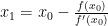
Introducing, Newton’s approximation for finding roots to a real-valued function (although it extends nicely to the complex plane, fortunately). For a function $f(x)$ and an initial “guess” $x_0$ , a better guess will be $x_1 = x_0 - \frac{f(x_0)}{f'(x_0)}$ , where $f'(x)$ is the derivative of $f(x)$ . In fact, this can be generalized to the recursive formula $x_{n+1} = x_n - \frac{f(x_n)}{f'(x_n)}$ . So how do we make fractals?

Have a function $f(x)$ , a size $(w, h)$ and a resolution $r$ .
Assign a unique color to each root to $f(x)$ .
For every point $P(x, y)$ in the image, make an inital guess $x_0 = (-r + (\frac{x}{w}) \cdot 2r, (-r + \frac{y}{h}) \cdot 2r)$ .
Use Newton’s approximation method to approximate a root as long as $x_{n+1} - x_n > \epsilon$ .
Color the pixel $P(x, y)$ the color which is assigned to the root which has just been approximated.